Step Response of a Second-Order System

File: examples/basic/01_step_response/step_response.py

---

What this example shows

The simplest possible Synapsys program: build a transfer function, compute its step response, and plot it. This is the "hello world" of control systems.

---

Theory

A transfer function $G(s)$ represents a linear time-invariant (LTI) system in the Laplace domain:

$$G(s) = \frac{Y(s)}{U(s)}$$

For a second-order underdamped system, the standard form is:

$$G(s) = \frac{\omega_n^2}{s^2 + 2\zeta\omega_n s + \omega_n^2}$$

Parameter	Symbol	Effect
Natural frequency	$\omega_n$	Controls oscillation speed
Damping ratio	$\zeta$	Controls how fast oscillations decay

Damping regimes:

• $\zeta < 1$ — underdamped: oscillates before settling
• $\zeta = 1$ — critically damped: fastest non-oscillating response
• $\zeta > 1$ — overdamped: slow, no oscillation

The step response is the output when the input switches from 0 to 1 at $t=0$. It is the primary tool for characterising a system's dynamic behaviour.

---

System used

$$G(s) = \frac{100}{s^2 + 10s + 100} \qquad \omega_n = 10,\quad \zeta = 0.5$$

With $\zeta = 0.5$ the system is underdamped — it overshoots and oscillates before settling at $y = 1$.

---

Result

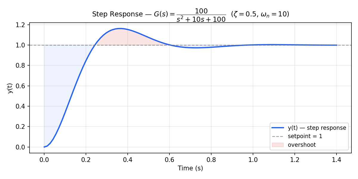
The shaded red region marks the overshoot (output exceeds the setpoint). The system settles within approximately $0.8\,\text{s}$.

---

Code

from synapsys.api.matlab_compat import tf, step
import matplotlib.pyplot as plt

wn, zeta = 10.0, 0.5
G = tf([wn**2], [1, 2*zeta*wn, wn**2])

print(G)
print(f"Poles   : {G.poles()}")
print(f"Stable  : {G.is_stable()}")

t, y = step(G)

plt.figure()
plt.plot(t, y, label="y(t)")
plt.axhline(1.0, color="k", linestyle="--", alpha=0.4, label="setpoint")
plt.title("Step Response — second-order system")
plt.xlabel("Time (s)")
plt.ylabel("y(t)")
plt.legend()
plt.grid(True)
plt.show()

Key API calls

Call	What it does
tf(num, den)	Builds a TransferFunction from coefficient lists (highest power first)
G.poles()	Returns roots of the denominator polynomial
G.is_stable()	True if all poles have negative real parts
step(G)	Computes step response via scipy.signal.step; returns (t, y)

---

How to run

uv run python examples/basic/01_step_response/step_response.py

Output: a plot window + step_response.png saved to the working directory.