Synapsys
A Python library for modelling, analysis and real-time simulation of linear control systems. Provides a MATLAB-compatible API over SciPy, a multi-agent simulation framework, and a pluggable transport layer (shared memory / ZMQ) for MIL → SIL → HIL workflows.
pip install synapsysuv add synapsysuv sync --extra devOverview
Synapsys covers the full control-design workflow — from continuous-time LTI modelling to discrete real-time closed-loop simulation — with a consistent API across all stages.
- LTI Models
- PID / LQR
- Real-Time Simulation
- AI Integration
from synapsys.api import tf, ss, step, bode, feedback, c2d

# Transfer function:  G(s) = ωn² / (s² + 2ζωnˢ + ωn²)
wn, zeta = 10.0, 0.5
G = tf([wn**2], [1, 2*zeta*wn, wn**2])

# Closed-loop (negative feedback)
T = feedback(G)

# Frequency and time-domain analysis
w, mag, phase = bode(G)
t, y          = step(T)

# Zero-order-hold discretisation at 200 Hz
Gd = c2d(G, dt=0.005)
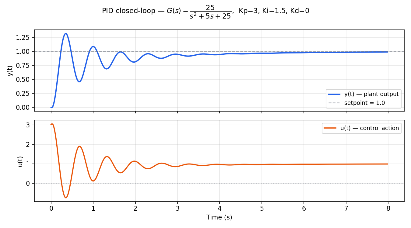
from synapsys.algorithms import PID, lqr
import numpy as np

# Discrete PID with anti-windup saturation
pid = PID(Kp=3.0, Ki=0.5, Kd=0.1, dt=0.01,
          u_min=-10.0, u_max=10.0)
u = pid.compute(setpoint=5.0, measurement=y)

# LQR — solves the continuous algebraic Riccati equation
#   minimises  J = ∫ (x'Qx + u'Ru) dt
A = np.array([[ 0.,  1.], [-wn**2, -2*zeta*wn]])
B = np.array([[0.], [wn**2]])
K, P = lqr(A, B, Q=np.eye(2), R=np.eye(1))
# Control law:  u = −Kx
from synapsys.api import ss, c2d
from synapsys.agents import PlantAgent, ControllerAgent, SyncEngine, SyncMode
from synapsys.algorithms import PID
from synapsys.transport import SharedMemoryTransport
import numpy as np

# Discretise G(s) = 1/(s+1)  at 100 Hz
plant_d = c2d(ss([[-1]], [[1]], [[1]], [[0]]), dt=0.01)

# Shared-memory bus — zero-copy, latency < 1 µs
with SharedMemoryTransport("demo", {"y": 1, "u": 1}, create=True) as bus:
    bus.write("y", np.zeros(1)); bus.write("u", np.zeros(1))

    pid = PID(Kp=4.0, Ki=1.0, dt=0.01)
    law = lambda y: np.array([pid.compute(setpoint=3.0, measurement=y[0])])

    sync = SyncEngine(SyncMode.WALL_CLOCK, dt=0.01)
    PlantAgent("plant", plant_d, bus, sync).start(blocking=False)
    ControllerAgent("ctrl",  law,     bus, sync).start(blocking=False)
import torch, torch.nn as nn, numpy as np
from synapsys.utils import StateEquations
from synapsys.algorithms import lqr
from synapsys.agents import ControllerAgent, SyncEngine, SyncMode
from synapsys.transport import SharedMemoryTransport

# ── 1. Build 2-DOF mass-spring-damper via named equations ──────────────────
m, c, k = 1.0, 0.1, 2.0
eqs = (
    StateEquations(states=["x1", "x2", "v1", "v2"], inputs=["F"])
    .eq("x1", v1=1).eq("x2", v2=1)
    .eq("v1", x1=-2*k/m, x2=k/m, v1=-c/m)
    .eq("v2", x1=k/m, x2=-2*k/m, v2=-c/m, F=k/m)
)

# ── 2. Compute LQR optimal gains (solves Algebraic Riccati Equation) ───────
K, _ = lqr(eqs.A, eqs.B, Q=np.diag([1., 10., .5, 1.]), R=np.eye(1))
# K = [−0.38, 2.23, 0.42, 1.75]  →  u* = −K·x + Nbar·r

# ── 3. MLP initialized with LQR gains (physics-informed) ──────────────────
class NeuralLQR(nn.Module):
    def __init__(self, K, Nbar):
        super().__init__()
        self.Nbar = Nbar
        self.net = nn.Sequential(
            nn.Linear(4, 32), nn.Tanh(),  # hidden layers — trainable by RL
            nn.Linear(32, 16), nn.Tanh(),
            nn.Linear(16, 1),             # output layer ← LQR gains
        )
        with torch.no_grad():
            self.net[4].weight.data = torch.tensor(-K.reshape(1, -1))
    def forward(self, x):
        return self.net(x) + self.Nbar   # u = MLP(x) + Nbar·r

model = NeuralLQR(K, Nbar=3.535).eval()

# ── 4. Plug into ControllerAgent — works with any nn.Module ───────────────
def control_law(state: np.ndarray) -> np.ndarray:
    with torch.no_grad():
        u = model(torch.tensor(state, dtype=torch.float32).unsqueeze(0))
    return np.clip(u.numpy().flatten(), -20.0, 20.0)

transport = SharedMemoryTransport("sil_2dof", {"state": 4, "u": 1}, create=False)
agent = ControllerAgent("neural_lqr", control_law, transport,
                        SyncEngine(SyncMode.WALL_CLOCK, dt=0.01))
agent.start(blocking=True)   # or blocking=False for real-time plot
Simulation Fidelity Ladder
Synapsys is designed for incremental fidelity increases. Only the transport layer changes — the controller algorithm remains identical across all three stages.
See the HIL / SIL guide for a step-by-step migration example.
AI + Control Systems — Quadcopter MIMO Demo
Any PyTorch, Keras or JAX model plugs directly into a ControllerAgent via a single np.ndarray → np.ndarray callback. Below: a 12-state MIMO quadcopter controlled by a residual Neural-LQR (δu = −K·e + MLP(e)) — the MLP starts zeroed so the system launches as pure LQR and can be fine-tuned via RL without losing stability.
PyVista 3D window (50 Hz) — drone mesh, trajectory trail, reference curve and live HUD.
matplotlib telemetry (10 Hz) — x-y position, altitude, Euler angles and control deviations δu.
Full walkthrough: Quadcopter MIMO Neural-LQR example →
3D Simulation Views
Janelas de simulação 3D prontas para usar — conecte qualquer controlador (LQR, PID, rede neural, agente RL) com uma única linha de código.
x = [x, ẋ, θ, θ̇]Inverted pendulum on a cart. 4 states, unstable — the classic benchmark for LQR and RL.
x = [θ, θ̇]Single-link pendulum on a fixed base. The simplest unstable system for testing any controller.
x = [q, q̇]Mass-spring-damper with setpoint tracking. LQR with position feed-forward.
Pass any callable as a controller — LQR, PID, neural network or RL agent: CartPoleView(controller=my_model).run() · See examples →
From the Blog
In-depth research articles and practical posts on control systems, AI and Synapsys.
PID with Anti-Windup: Theory, Tuning and Experimental Validation
A research-oriented deep-dive into discrete PID with back-calculation anti-windup — from the integral windup problem to experimental step-response validation, with Synapsys code throughout.
Read full article →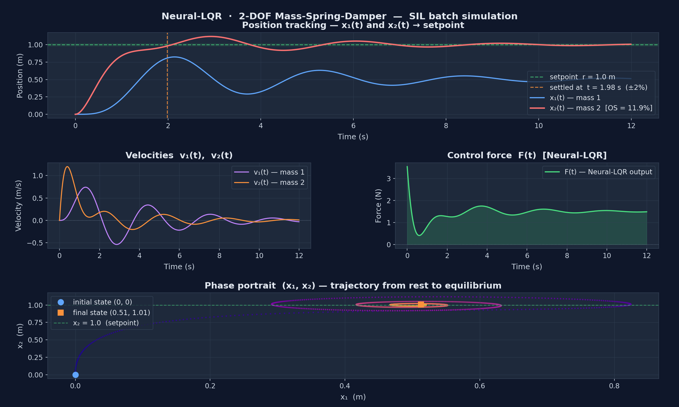
From Model to Hardware: MIL → SIL → HIL in Three Steps
A practical guide to the MIL/SIL/HIL development workflow with Synapsys — swap from simulation to real hardware by changing one line, keeping your control algorithm untouched.
Read full article →PID with Anti-Windup: Theory, Tuning and Experimental Validation
A research-oriented deep-dive into discrete PID with back-calculation anti-windup — from the integral windup problem to experimental step-response validation, with Synapsys code throughout.
Read full article →Full Library Map
Nine focused packages — from LTI mathematics to real-time hardware. Click any card to jump to the API reference.
MATLAB-Compatible API
Familiar entry point — mirrors the MATLAB Control Toolbox interface.
Core LTI Systems
Mathematical backbone — transfer functions, state-space and MIMO matrices.
Control Algorithms
Discrete PID with anti-windup and LQR via the Algebraic Riccati Equation.
Multi-Agent Simulation
Lifecycle agents for real-time closed-loop simulation with lock-step or wall-clock sync.
Message Broker
High-level pub/sub bus decoupled from the transport layer — shared memory or ZMQ backend.
Transport Layer
Zero-copy IPC and networked PUB/SUB for distributed MIL → SIL → HIL workflows.
Utilities
Matrix builders and declarative state-equation DSL for clean model definitions.
Hardware Interface
Abstract interface for FPGA, FPAA and microcontroller backends — planned for v0.5.
State Observers
Kalman filter and Luenberger observer for state estimation — planned for v0.3.
Package Overview
| Package | Contents | Status |
|---|---|---|
synapsys.core | TransferFunction, StateSpace, ZOH discretisation | Stable |
synapsys.api | MATLAB-compatible layer: tf(), ss(), step(), bode() | Stable |
synapsys.algorithms | Discrete PID with anti-windup, LQR (ARE solver) | Stable |
synapsys.agents | PlantAgent, ControllerAgent, SyncEngine | Functional |
synapsys.transport | SharedMemory (zero-copy), ZMQ PUB/SUB & REQ/REP | Functional |
synapsys.viz | 3D sim views plug-and-play: CartPoleView, PendulumView, MassSpringDamperView | Functional |
synapsys.hw | HardwareInterface, MockHardwareInterface (HIL) | Interface |
synapsys.mpc | Model Predictive Control | Planned |