Quick Start

This guide walks through the five core workflows of Synapsys — from a single transfer function to a full distributed closed-loop simulation. Each section builds on the previous one.

Prerequisites

Install Synapsys before starting: pip install synapsys or uv add synapsys

---

1. Analysing a Continuous-Time System

A transfer function $G(s)$ describes how a linear time-invariant (LTI) system transforms an input $U(s)$ into an output $Y(s)$ in the Laplace domain:

$G(s) = \frac{Y(s)}{U(s)} = \frac{\omega_n^2}{s^2 + 2\zeta\omega_n s + \omega_n^2}$

Key parameters:

• $\omega_n$ — natural frequency: how fast the system oscillates (rad/s)
• $\zeta$ — damping ratio: how quickly oscillations decay (0 < ζ < 1 → underdamped)

The step response — output when the input jumps from 0 to 1 at $t=0$ — reveals the dynamic behaviour: overshoot, rise time, and settling time.

from synapsys.api import tf, step
import matplotlib.pyplot as plt

# G(s) = ωn² / (s² + 2ζωn·s + ωn²)
wn, zeta = 10.0, 0.5
G = tf([wn**2], [1, 2*zeta*wn, wn**2])

# Inspect the system
print(f"Poles:      {G.poles()}")      # complex conjugate pair
print(f"DC gain:    {G.evaluate(0).real:.4f}")   # G(0) = 1.0
print(f"Stable:     {G.is_stable()}")  # True — all poles in left half-plane

# Compute and plot step response
t, y = step(G)

plt.figure(figsize=(9, 4))
plt.plot(t, y, label="y(t)")
plt.axhline(1.0, color="gray", ls="--", alpha=0.6, label="setpoint")
plt.xlabel("Time (s)"); plt.ylabel("y(t)")
plt.title("Step Response"); plt.legend(); plt.grid(True)
plt.show()

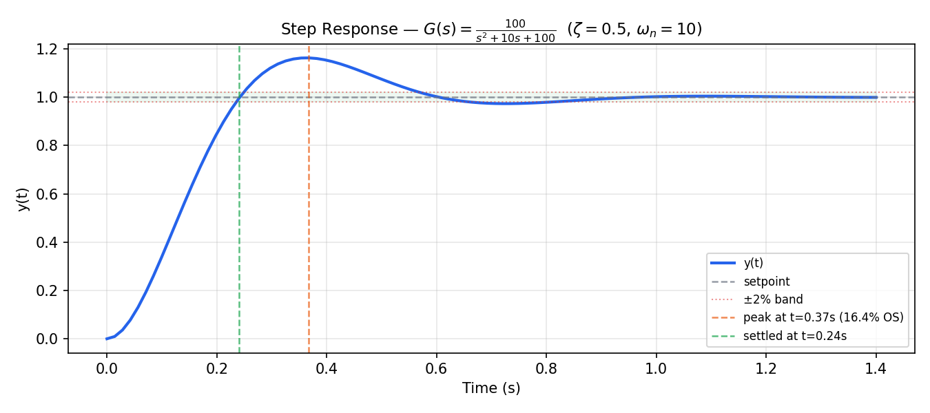
The system overshoots by ~16.4% and settles (within ±2% of the setpoint) at ~0.24 s. Both are directly predictable from $\zeta = 0.5$:

$\text{Overshoot} = e^{-\pi\zeta/\sqrt{1-\zeta^2}} \approx 16.3\%$

---

2. Closed-Loop with Unity Negative Feedback

An open-loop system amplifies the input but cannot reject disturbances or correct steady-state error. Closing the loop with negative feedback trades some gain for stability and disturbance rejection.

For a plant $G(s)$ with unity negative feedback, the closed-loop transfer function is:

$T(s) = \frac{G(s)}{1 + G(s)}$

from synapsys.api import tf, feedback, step

G = tf([10], [1, 1])       # G(s) = 10/(s+1)  — DC gain = 10
T = feedback(G)            # T(s) = 10/(s+11) — DC gain = 10/11 ≈ 0.909

print(f"Open-loop  DC gain: {G.evaluate(0).real:.4f}")   # 10.0
print(f"Closed-loop DC gain: {T.evaluate(0).real:.4f}")  # 0.9091

t, y = step(T)

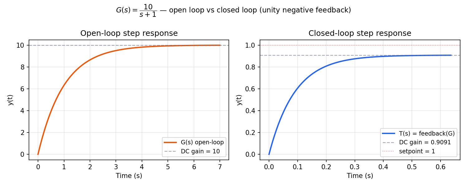
Open-loop (left): the output rises to 10× the input and settles slowly — no reference tracking, just amplification.

Closed-loop (right): feedback(G) reduces the DC gain to $\frac{10}{1+10} \approx 0.909$. This residual error ($\approx 9\%$) is the steady-state error inherent to a proportional-only loop. Adding an integrator (see section 4) eliminates it.

feedback() API

feedback(G) computes G/(1+G).
feedback(G, C) computes the loop G·C/(1+G·C) with controller C in the forward path.

---

3. Discretisation

Real controllers run on digital hardware at a fixed sampling rate. c2d converts a continuous model to a discrete one using Zero-Order Hold (ZOH) — assuming the control input $u$ is constant between samples:

$G_d(z) = \mathcal{Z}\left\{G(s) \cdot \frac{1 - e^{-sT_s}}{s}\right\}$

Choosing the right sampling period $T_s$ is critical:

• Too slow ($T_s$ large): aliasing, poor approximation of the continuous dynamics
• Too fast ($T_s$ small): unnecessary computation, numerical issues
• Rule of thumb: $T_s \leq \frac{1}{10 f_{\text{bandwidth}}}$ — sample at least 10× the system bandwidth

from synapsys.api import tf, c2d, step

G = tf([1], [1, 2, 1])        # G(s) = 1/(s+1)² — continuous

Gd_fast = c2d(G, dt=0.05)     # 20 Hz — well above bandwidth
Gd_slow = c2d(G, dt=0.5)      # 2 Hz — too coarse

print(f"Discrete (fast): {Gd_fast.is_discrete}")  # True
print(f"Stable:          {Gd_fast.is_stable()}")   # True

# Step response — 200 samples
t_fast, y_fast = step(Gd_fast, n=200)
t_slow, y_slow = step(Gd_slow, n=20)

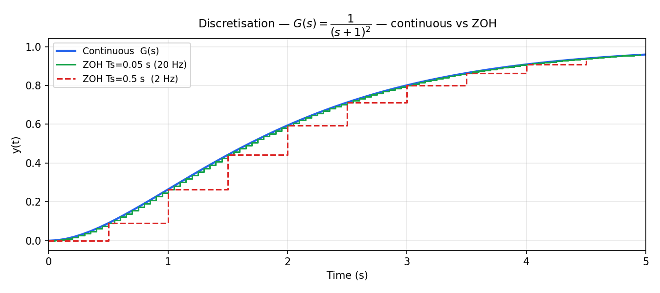
At 20 Hz (green) the discrete response is virtually identical to the continuous one. At 2 Hz (red dashed) the ZOH staircase is clearly visible — the output holds each sample until the next tick.

---

4. PID Control

A PID controller computes the control action from three terms:

$u(t) = K_p\,e(t) + K_i\int_0^t e(\tau)\,d\tau + K_d\,\dot{e}(t)$

where $e(t) = r(t) - y(t)$ is the tracking error.

Term	Effect	Tuning
$K_p$ (proportional)	Speed of response	Higher → faster, but more overshoot
$K_i$ (integral)	Eliminates steady-state error	Higher → faster correction, but more overshoot/oscillation
$K_d$ (derivative)	Damps oscillations	Higher → smoother, but sensitive to noise

Synapsys provides a discrete PID with anti-windup saturation — the integrator is clamped to [u_min, u_max] to prevent integrator windup when the actuator saturates.

from synapsys.api import tf, c2d
from synapsys.algorithms import PID
import numpy as np

DT = 0.02
plant_d = c2d(tf([25], [1, 5, 25]), dt=DT)   # G(s) = 25/(s²+5s+25)
pid     = PID(Kp=3.0, Ki=1.5, Kd=0.0, dt=DT, u_min=-10.0, u_max=10.0)

SETPOINT = 1.0
x = np.zeros(plant_d.n_states)

for _ in range(400):
    x, y_arr = plant_d.evolve(x, np.array([u]))   # advance plant one step
    y = float(y_arr[0])
    u = pid.compute(setpoint=SETPOINT, measurement=y)

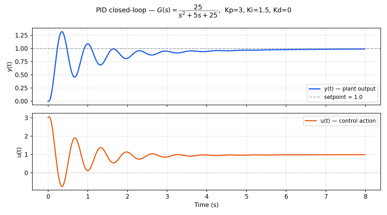
The integral term eliminates the steady-state error seen in section 2 — y(t) converges exactly to the setpoint. The control signal u(t) starts large (high initial error) and decays to a small value that compensates for the plant's finite DC gain.

Tuning starting point

For a second-order underdamped plant, start with $K_i \approx K_p / 3$ and $K_d = 0$. Add $K_d$ only if overshoot is too large.

---

5. Distributed Simulation (Same Machine)

Synapsys can split the plant and controller into separate processes communicating via zero-copy shared memory — mimicking a real embedded system where the plant (PLC/sensor) and controller (computer) run independently.

Run in two separate terminals:

# Terminal 1 — start the plant first
python examples/distributed/01_shared_memory/plant.py

# Terminal 2 — then the controller
python examples/distributed/01_shared_memory/controller.py

The plant exposes its state via shared memory (zero-copy, latency < 1 µs). The controller reads y, computes u with PID, and writes it back — no network sockets involved.

---

6. Distributed Simulation (Different Machines)

For cross-machine simulation, use ZeroMQ as the transport layer. The plant publishes y over TCP and subscribes to u; the controller does the reverse.

# Machine A — plant
python examples/distributed/02_zmq/plant_zmq.py

# Machine B — controller (set PLANT_HOST to Machine A's IP)
PLANT_HOST=192.168.1.10 python examples/distributed/02_zmq/controller_zmq.py

Both processes can run on the same machine for local testing — just open two terminals.

---

Next steps

• Examples → — runnable scripts for every pattern (SIL, Digital Twin, Real-Time Oscilloscope, AI controller)
• User Guide → — deep dive into LTI models, PID, LQR, agents and transport
• API Reference → — complete class and function reference