Real-Time Oscilloscope with Sinusoidal Reference

File: examples/advanced/04_realtime_oscilloscope/04_realtime_matplotlib.py

---

What this example shows

The most complete self-contained real-time simulation in Synapsys. Three concurrent roles — plant, controller, and oscilloscope — run simultaneously without blocking each other.

The control objective is sinusoidal reference tracking: the setpoint is a time-varying signal and the PID must keep the output following it continuously.

---

Architecture

The plant and controller run in background threads (blocking=False). The main thread drives the FuncAnimation loop.

---

Sinusoidal reference

$$r(t) = 3 + 2\sin(2\pi \cdot 0.2 \cdot t)$$

A 0.2 Hz (5-second period) sinusoid with DC offset 3. The PID must compute u(t) at every tick so that y(t) ≈ r(t) despite plant dynamics introducing a phase lag.

The reference is evaluated from wall-clock time via a closure:

t_start = time.monotonic()

def law(y):
    r = SP_OFFSET + SP_AMP * np.sin(2 * np.pi * SP_FREQ * (time.monotonic() - t_start))
    return np.array([pid.compute(setpoint=r, measurement=y[0])])

Each call to law(y) reads the current time, computes r(t), and feeds it to the PID — no external coordination needed.

---

Rolling window oscilloscope

WINDOW = 200   # samples (200 × 0.02 s = 4 s visible)
buf_t = deque([0.0] * WINDOW, maxlen=WINDOW)
buf_y = deque([0.0] * WINDOW, maxlen=WINDOW)

deque(maxlen=N) automatically discards the oldest sample when a new one is appended. The x-axis scrolls forward:

x_min = max(0.0, now - WINDOW * DT)
x_max = x_min + WINDOW * DT
ax.set_xlim(x_min, x_max)

---

PID tuning

pid = PID(Kp=6.0, Ki=2.0, dt=DT, u_min=-15.0, u_max=15.0)

Parameter	Value	Rationale
Kp	6.0	Fast proportional response for sinusoidal tracking
Ki	2.0	Eliminates the phase-lag-induced steady-state error
u_min/max	±15	Anti-windup saturation

---

Result

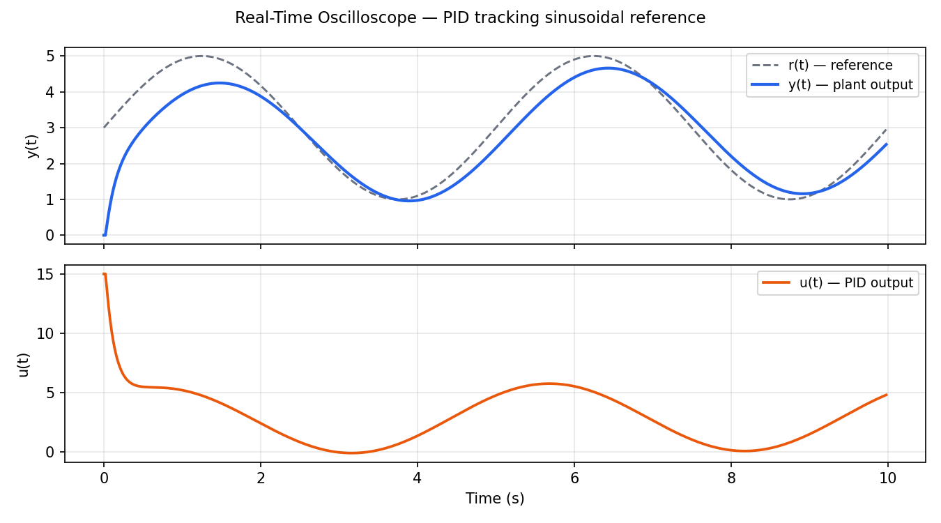
y(t) (blue) tracks r(t) (dashed) with a small phase lag introduced by the plant dynamics. u(t) (orange) oscillates as the PID continuously compensates — amplitude grows when tracking error grows (bottom of the sine) and shrinks when the error is small.

---

How to run

Single terminal — everything runs in-process:

uv run python examples/advanced/04_realtime_oscilloscope/04_realtime_matplotlib.py

The oscilloscope window opens immediately. Close it to stop the simulation.