Digital Twin with Anomaly Detection
File: examples/advanced/05_digital_twin/05_digital_twin.py
What this example shows
The Digital Twin pattern: a virtual model of a physical system runs in parallel, fed with the same control inputs. When the physical system starts behaving differently from the model (due to wear or damage), the divergence metric triggers an alert.
Architecture
Theory
Why digital twins detect wear
At , both plant and twin have the same dynamics. The controller drives them to the same setpoint.
At (wear injection), the physical plant's pole shifts:
The worn plant responds twice as fast but to a different magnitude. The twin, still using , diverges from the physical output. The divergence metric:
grows past the alert threshold within a few ticks of the wear event.
Virtual twin evolution
The twin evolves in the main thread via evolve(), synchronised with each bus read:
# Observer reads directly from the broker — no extra transport handle needed
y_physical = broker.read("twin/y")[0]
u_current  = broker.read("twin/u")[0]

# Step the twin with the SAME u
x_virtual, y_virtual_arr = plant_nominal.evolve(
    x_virtual, np.array([u_current])
)
This guarantees that both the physical and virtual outputs are computed with the same u(t) — the only difference is the internal model.
Wear injection — hot swap
The plant model is swapped at runtime without stopping the controller or the bus:
if elapsed >= DRIFT_AT:
    plant_agent.stop()                              # graceful shutdown
    plant_agent = PlantAgent("worn", drifted_model, ...)
    plant_agent.start(blocking=False)               # restart with new model
The bus, controller, and virtual twin continue uninterrupted.
Result
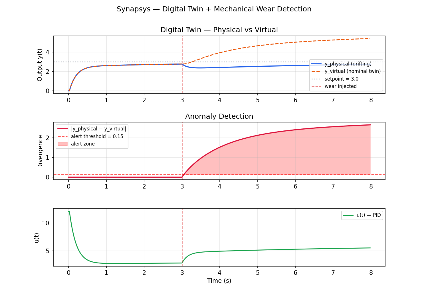
Panel 1 — Physical vs Virtual: outputs are identical until , then diverge.
Panel 2 — Anomaly Detection: the red fill shows ticks where . The alert zone grows steadily after the wear event.
Panel 3 — Control signal: the PID compensates more aggressively post-wear because the plant dynamics have changed.
Real-world applications
| Domain | Physical system | Wear signature |
|---|---|---|
| Industrial | Pump or motor | Increased damping, reduced efficiency |
| Aerospace | Control surface | Actuator stiffness change |
| Structural | Bridge or building | Natural frequency shift |
| Process control | Heat exchanger | Fouling increases thermal resistance |
How to run
Single terminal — runs for 8 seconds then plots:
uv run python examples/advanced/05_digital_twin/05_digital_twin.py
Expected terminal output:
[t=3.00s] Wear injected: plant pole drifted -1 -> -2
[t=3.05s] ALERT: divergence = 0.18 > 0.15
...
Simulation complete. N ticks with divergence > 0.15.
Source
| File | Description |
|---|---|
examples/advanced/05_digital_twin/05_digital_twin.py | Complete example — physical plant, virtual twin, PID, wear injection, divergence monitoring, 3-panel plot |