Custom Signal Injection (MIL / Batch Simulation)

File: examples/advanced/01_custom_signals/01_custom_signals.py

---

What this example shows

How to feed any arbitrary waveform into an LTI model and observe the output — without real-time constraints. This is Model-in-the-Loop (MIL) simulation: everything runs in software, as fast as the CPU allows.

The example also visually demonstrates the principle of superposition: the response to a combined input equals the sum of individual responses.

---

Theory

MIL vs SIL vs HIL

Mode	Plant	Controller	Real-time
MIL	Math model	Math model	No — runs at CPU speed
SIL	Math model (real-time)	Real software	Yes
HIL	Real hardware	Real software	Yes

MIL is ideal for batch testing, parameter sweeps, and signal analysis.

Principle of Superposition

For any linear system $G(s)$:

$$G(u_1 + u_2) = G(u_1) + G(u_2)$$

This example combines:

1. A 1.5 Hz sine wave — simulating periodic mechanical vibration
2. A step of amplitude 2 at $t=5\,\text{s}$ — simulating a sudden load change

---

System used

$$G(s) = \frac{10}{s^2 + 5s + 10} \qquad \omega_n = \sqrt{10} \approx 3.16\,\text{rad/s},\quad \zeta \approx 0.79$$

Well-damped (close to critically damped) — attenuates the sine and responds smoothly to the step.

---

Result

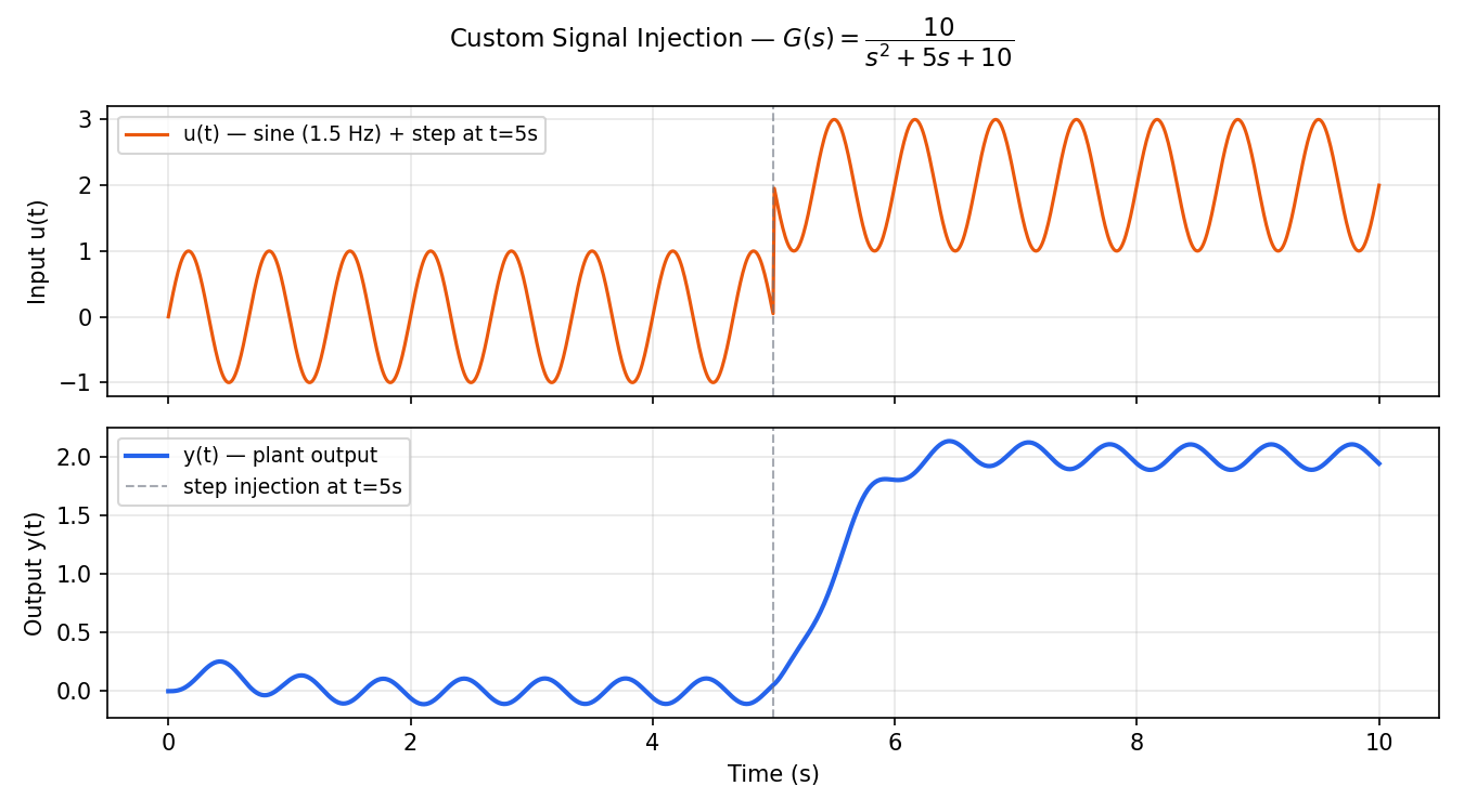
Top panel: the combined input $u(t)$ = sine + step. The vertical line marks $t=5\,\text{s}$ when the step is injected.

Bottom panel: the plant output $y(t)$. The DC level shifts upward after $t=5\,\text{s}$ while the oscillation from the sine continues — superposition in action.

---

Code

import numpy as np
from synapsys.api import tf
import matplotlib.pyplot as plt

G = tf([10], [1, 5, 10])

t = np.linspace(0, 10, 1000)

# 1.5 Hz mechanical vibration
u_sine = np.sin(2 * np.pi * 1.5 * t)

# Step disturbance at t = 5 s
u_step = np.where(t >= 5, 2.0, 0.0)

# Superposition
u_total = u_sine + u_step

t_out, y_out = G.simulate(t, u_total)

plt.plot(t_out, u_total, label="Input u(t)")
plt.plot(t_out, y_out, label="Output y(t)", linewidth=2)
plt.legend()
plt.show()

Key API calls

Call	What it does
tf(num, den)	Builds the LTI transfer function
G.simulate(t, u)	Computes output for arbitrary input array u over time t via scipy.signal.lsim
np.where(cond, a, b)	Vectorised conditional — creates the step signal efficiently

---

How to run

uv run python examples/advanced/01_custom_signals/01_custom_signals.py